Outlook: A Stock Trend Predictor

Outlook is a learned indicator of an asset's medium-term price trend. I developed it to predict whether the price is likely to remain above or below its current level over a future interval, with greater importance assigned to nearer observations. The model learns a weighted summary of that interval from historical price indicators.

In my experiments, using Outlook to guide transactions outperformed holding individual assets in non-bullish markets. Applied across collections of assets, it also outperformed capitalization-weighted benchmarks across the market conditions evaluated. The method begins with the prediction target: a time-weighted average of future price changes that gives the network a numerical definition of the trend it should learn.

1. Choosing what to predict

Consider two price paths that start at the same price and finish at the same price a month later. One rises early and stays elevated for most of the month; the other falls before recovering near the end. A forecast of the final price assigns them the same target. For a strategy that can enter and exit during the interval, their differences matter.

Predicting the whole path would retain those differences, though it would also require the model to estimate many future values from a limited history. Daily observations for a single asset provide relatively few training examples, especially when the feature windows overlap. A more compact target lets the model learn the direction and persistence of the future movement without estimating every point along it.

I use a weighted average of future displacements from the current price. This preserves information about how long a move lasts and when it occurs, while keeping the output scalar. Choosing the target and loss together also makes the forecasting objective explicit, following the distinction between forecast quantities and scoring functions discussed by Gneiting. 1

2. The Outlook target

Let $P_t$ denote the adjusted asset price at observation $t$, and let $N$ be the forecast horizon in trading observations. Define

$$O_t=\frac{1}{Z_N}\sum_{i=1}^{N}w_i(P_{t+i}-P_t), \qquad Z_N=\sum_{i=1}^{N}w_i.$$

The weights are nonnegative and decrease with the delay $i$. Dividing by their sum keeps the target in price units. If $O_t=5$, the weighted future price is five units above the price at $t$. Negative values indicate that it lies below the starting price.

For a persistent increase, many terms in the sum are positive. A short-lived spike affects fewer terms and contributes less to the average. This is the behavior I wanted the indicator to capture: how the price develops throughout the holding window, including the persistence of a move.

Weighting the horizon

A uniform average gives the final included observation the same weight as the first, followed by an abrupt drop to zero outside the window. I use a quadratic taper:

$$w_i=1-\left(\frac{i}{N}\right)^2, \qquad 1\leq i\leq N,\quad N\geq2.$$

The weight starts near one and falls to zero at the horizon. At one-quarter, one-half, and three-quarters of the horizon, the corresponding weights are $15/16$, $3/4$, and $7/16$. Much of the interval retains substantial influence, with observations near the endpoint contributing progressively less.

Extending the function by zero beyond $N$ gives a continuous transition at the boundary. The target remains defined over a finite window; the taper removes the jump in weight that a uniform window would introduce there.

The discrete normalizing constant is

$$\begin{aligned} Z_N &=N-\frac{1}{N^2}\sum_{i=1}^{N}i^2\\ &=N-\frac{(N+1)(2N+1)}{6N}\\ &=\frac{(N-1)(4N+1)}{6N}. \end{aligned}$$

For comparison, integrating the continuous weight over the horizon gives $2N/3$. Normalization separates the shape of the weighting function from its total mass, so the interpretation of $O_t$ remains a weighted price displacement.

The implied weight on daily changes

The effect of an early move can be seen by expanding each displacement into individual price changes. Write $\Delta P_{t+j}=P_{t+j}-P_{t+j-1}$. Then

$$\begin{aligned} O_t &=\frac{1}{Z_N}\sum_{i=1}^{N}w_i \sum_{j=1}^{i}\Delta P_{t+j}\\ &=\sum_{j=1}^{N}\beta_j\Delta P_{t+j}, \qquad \beta_j=\frac{\sum_{i=j}^{N}w_i}{Z_N}. \end{aligned}$$

The first change enters every future displacement, giving it a coefficient of one. A later change enters only the displacements after it occurs. An increase early in the interval therefore contributes more than the same increase near the end, even if both paths eventually reach the same price.

Raw Outlook values scale with the asset's price. Multiplying the entire price series by a constant multiplies $O_t$ by that constant as well. The training pipeline normalizes the target before fitting the network, and the final activation bounds the estimated signal between $-1$ and $1$.

3. Representing the price history

I construct the inputs from moving averages, standardized price deviations, and volatility-related features at several window lengths. The moving average for a window of $k$ observations is

$$\mu_t^{(k)}=\frac{1}{k}\sum_{j=0}^{k-1}P_{t-j}.$$

Short windows respond quickly to a change in price; longer windows retain more of the preceding trajectory. A standardized deviation describes the current price's distance from its local average relative to dispersion, while the volatility-related stream supplies information about the size of recent fluctuations.

The model receives histories of these indicators rather than only their most recent values. For example, two observations can have the same current moving average after very different sequences of increases and decreases. Keeping the preceding indicator values makes those histories available to the model.

The configuration uses 5- and 10-observation feature windows with 200 observations of history. Concatenating three streams at both window lengths produces a 1,200-dimensional input. Each feature history is normalized before being passed to the network.

4. Residual regression model

The network begins with a 256-unit dense layer and ReLU activation, followed by batch normalization and dropout. Two residual blocks expand this representation to 512 units, project it back to 256, and add the input to the block output:

$$h_{\ell+1}=h_\ell+F_\ell(h_\ell).$$

This follows the residual formulation of He et al. 2 The identity path carries the current representation through the block, allowing the learned branch to modify it. Keeping both paths at width 256 makes their outputs directly compatible for addition.

Dense layers of widths 128 and 64 then reduce the representation before a scalar output layer:

$$\widehat y_t=\tanh(w^\top h_t+b).$$

Batch normalization is used between hidden transformations, and dropout randomly suppresses activations during training with a rate of 0.3 at the configured layers. These components follow Ioffe and Szegedy's normalization method and Srivastava et al.'s dropout procedure. 3 4

The network is trained with mean absolute error on the normalized Outlook labels:

$$\mathcal L(\theta)=\frac{1}{m}\sum_{t\in\mathcal T} \left|f_\theta(x_t)-y_t\right|.$$

Absolute-error loss targets a conditional median of the label distribution. 1 Accordingly, the output estimates the normalized weighted trend associated with the observed feature history. Its scale comes from the target normalization; it should be read as a trend signal rather than a percentage return.

Optimization uses Adam, which maintains first- and second-moment estimates of the gradients to adapt parameter updates. 5 The training configuration uses a learning rate of $10^{-3}$ and 30 epochs.

5. Results

I evaluated Outlook at two levels: using the signal to trade individual assets, and applying it across a collection of assets against a capitalization-weighted benchmark. The individual-asset experiments outperformed holding the asset in non-bullish markets. Across asset collections, Outlook outperformed the capitalization-weighted benchmark in the market conditions tested.

The single-asset chart below shows the price in blue and predicted Outlook on the right axis. Green triangles mark purchases and red triangles mark sales. The signal stays elevated through sustained upward movements and falls ahead of or during drawdowns, providing information for entry and exit decisions.

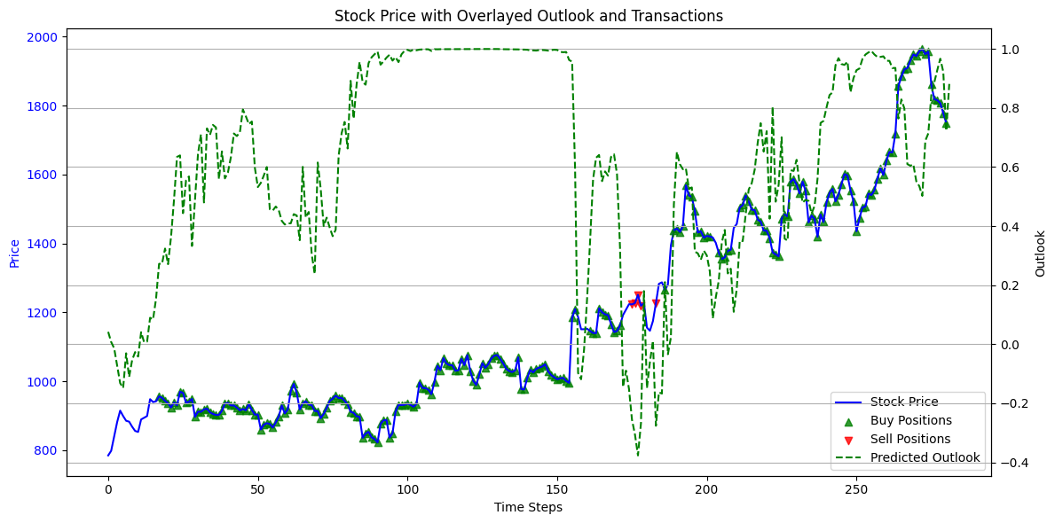
The target's preference for persistent movement helps explain the role of the indicator. An isolated favorable observation has limited weight, while a sequence of prices above the entry level contributes repeatedly. The learned signal can therefore remain positive through small reversals within an otherwise favorable interval.

For an individual asset, the strategy uses that signal to adjust exposure over time. Across a collection, the same model structure can be trained on each asset's history, producing signals that guide transactions throughout the portfolio. These evaluations test whether the estimated trend is useful for investment decisions in addition to whether it matches the supervised labels.

6. Further experiments

The next step is to test additional features and investigate whether related assets can contribute useful training information. Stocks within an industry may share responses to common conditions, so pooling their histories could increase the available training sample. Correlation analysis would help identify which groups are worth testing, while per-asset normalization would control differences in price scale.

I also want to extend the evaluation to the S&P 500 with more compute. The existing collection-level results motivate that larger experiment. Keeping the target and model fixed during the expansion would make it easier to examine how performance changes with the breadth of the asset universe.

References

1. Tilmann Gneiting. Making and Evaluating Point Forecasts. Journal of the American Statistical Association, 106(494):746–762, 2011.
2. Kaiming He, Xiangyu Zhang, Shaoqing Ren, and Jian Sun. Deep Residual Learning for Image Recognition. CVPR, 2016.
3. Sergey Ioffe and Christian Szegedy. Batch Normalization: Accelerating Deep Network Training by Reducing Internal Covariate Shift. ICML, 2015.
4. Nitish Srivastava, Geoffrey Hinton, Alex Krizhevsky, Ilya Sutskever, and Ruslan Salakhutdinov. Dropout: A Simple Way to Prevent Neural Networks from Overfitting. Journal of Machine Learning Research, 15(56):1929–1958, 2014.
5. Diederik P. Kingma and Jimmy Ba. Adam: A Method for Stochastic Optimization. ICLR, 2015.